Covariance and contravariance on manifolds
Explained also in covariance and contravariance in linear algebra.
If we have two charts for the same region of a manifold $M$, denoted $x$ and $y$, related through a transformation
$$ \phi: x \to y $$the matrix
$$ d \phi=\frac{\partial y^b}{\partial x^a} $$is the one that converts the coordinates of the tangent space vectors in the base provided by $x$ to the coordinates of the base provided by $y$.
But $d \phi$ and $d \phi^{-1}$ are not just changes of coordinates, they can also be interpreted as a transformation of vectors (this occurs from the level of linear algebra, matrices can be base changes or transformation of space, *if we leave the second base fixed*). However, then, the matrix that transforms the base provided by the chart $x$ into the base provided by $y$ is not $d\phi$, but
$$ d \phi^{-1}=\frac{\partial x^a}{\partial y^b} $$Moreover, if to transform the coordinates of the vectors from chart $x$ into the coordinates in $y$ we have used column matrices and the matrix multiplied the vector from the left, to convert vectors from the base of chart $x$ into those of the base of chart $y$ we use row matrices (although internally they are vectors) and multiplication from the right. This can be switched to the comfortable form (columns and multiplication from the left) by taking the transpose.
So, the matrix to transform one into the other is:
$$ d \left(\phi^{-1} \right)^t=\left(\frac{\partial x^a}{\partial y^b} \right)^t $$That is, vectors themselves transform in one direction, but their coordinates transform in the opposite direction. Hence the name contravariance.
It's somewhat analogous to what happens when we change the time. If we advance our clock, our temporal coordinate is at +1 but we are actually moving backwards (-1) because at the same hour as yesterday it is now earlier (there's more light).
Summing up:
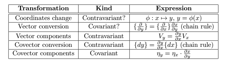
More over:
Let's restrict to 2D case. When we have a vector, say
$$ 2\partial x+\partial y $$and a covector
$$ dx+3dy $$we can represent them like an arrow, the first one, and a gradient (at least locally), the second one
The application of one into the other is the number of lines of the gradient that cross the vector. This is because to count the crossing lines we can count first in the horizontal direction and then add those from the vertical direction. See visualization of k-forms.
The gradient produced by, for example, $dx+3dy$ corresponds to a line trough the point $(0,1/3)$ and $(1,0)$, its parallel line through the $(0,0)$ and others at the same distance. Why the 3 produces 1/3? It has to do with real examples:
1) imagine vectors are stock in a shop and covectors are prices, a cost, a barrier, to every product in the shop.
2) a covector is a frequency, a vector is like a wavelength, and their product is analogous to a velocity (no estoy seguro de esto, es copiado de aquí y creo que se le puede sacar más partido a la analogía, viendo lo que pasa en la exponencial soluciión de la ecuación de onda multidimensional).
Observe that the set of parallel lines is perpendicular to the vector (arrow) $(1,3)=\partial x+ 3 \partial y$. The similitud with the original $dx+3dy$ is not coincidence: it is the covariant version of the other. It is exactly the same because in this case we are assuming the trivial metric
$$ \left( \begin{array}{cc} 1 & 0 \\ 0 & 1 \end{array} \right) $$What if we were with the metric
$$ \left( \begin{array}{cc} 4 & 0 \\ 0 & 1 \end{array} \right) $$ ?The covector $dx+3dy$ would be coming from the vector $1/4 \partial x+3\partial y$, that is still orthogonal to the parallel line but with the new concept of orthogonality.
Now consider a change of basis, a clockwise rotation of angle $\theta$, $R_{\theta}$, for example. It is a passive change, in the sense that we transform our basis but the main characters, the arrow and the gradient, are the same.
The new basis is obtained by applying the matrix $R_{\theta}$ through the right side or with the transpose of $R_{\theta}$ in the usual side (i.e., is covariant). But how i expressed now the vector $2 \partial x+\partial y$? You can check that you have to multiply $R_{-\theta}$ to the components! This is why vectors are called contravariant vectors.
And what about the gradient? Now, you can check that the line appears rotated and correspond to a different covector. The new components can be obtained by multiplying by $R_{\theta}$ in the right side, just like the vector conversion! So they are called covariant vectors.
And even more about contra and covariance
In a shop, imagine we have a product, apples, whose amount we measure in kg. The price is measured in eur/kg. When somebody comes to the shop and buys 4 kg of apples with a price of 2'5 eur/kg, he does the simple computation:
$$ 4 \cdot 2'5=10 $$to obtain an scalar. It could be done with several items and several prices, but we always obtain a scalar.
But, what if we change the units in which we measure the apples. For example, imagine that apples are sold in packets of 2'3 kg. Observe:
- The unit itself has been multiplied by 2'3 (kg to packet).
- The quantity of apples bought is no longer 4, but less than 4. It is divided by 2'3, for which we say is contravariant.
- The price is no longer 2'5, but it change to a greater price. It is multiplied by 2'3. So it is called covariant.
- The fact is that we obtain the same scalar: the total money.
- Everything works well if we replace apple with a list of products and a list of prices: vectors and covectors.
________________________________________
________________________________________
________________________________________
Author of the notes: Antonio J. Pan-Collantes
INDEX: